SPSS Exercises
Computing Analysis of Variance Models
Social scientists have examined the association between a woman’s fertility decisions (deciding whether and/or when to have a child) and her wages, employment status, and education, along with other socioeconomic and demographic factors. Research has indicated that different social groups may have different norms and values about fertility.
In this example, we’ll investigate the relationship between a woman’s educational attainment and the age at which her first child was born using GSS2014SSDS-A. We first analyzed this relationship in chapter 4, exercise 8. Using education as the independent variable and age at which her first child was born as the dependent variable, we can assess whether there is a relationship between educational attainment and age at first childbirth.
We’ll use two variables for our analysis, the variable DEGREE (five categories of educational attainment) and AGEKDBRN (respondent’s age when her first child was born). But first, we’ll restrict our analysis to women in the GSS sample (using Data—Select Cases command. You will have to select the option “If the condition is satisfied,” then type SEX = 2 to restrict your analysis to women).
We can compute the ANOVA model by clicking on Analyze, Compare Means, then One-Way ANOVA. The opening dialog box requires that we insert AGEKDBRN in the box labeled “Dependent List” and in the box labeled “Factor” insert DEGREE.
Click on the Options button at the upper right. Click on Descriptive in the Statistics box. This will produce a table of means and standard deviations along with the ANOVA statistics. Click on Continue in the Options box, then click OK in the One-Way ANOVA box.
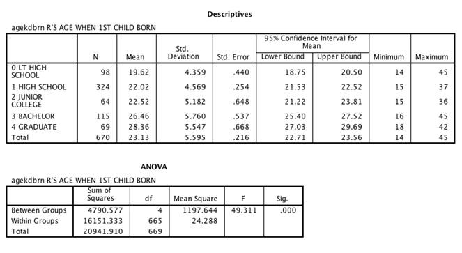
We are interested in the F statistic and significance in the ANOVA table (Figure 10.1). Based on the output, F is 49.311 significant at the .000 level. The data reveal a positive relationship--the higher one’s educational attainment, the higher the age of first childbirth. The oldest average age at first childbirth is for women with graduate degrees (28.36 years of age), followed by women with bachelor’s degrees (26.46 years of age). The youngest group of first-time mothers is women with less than a high school diploma. On average, women with less than a high school diploma had their first child at 19.62 years of age. When compared with the age of graduate-degree first-time mothers, there is a difference of 8.74 years.
Figure 10.1. ANOVA Output for Age at First Childbirth and Education, Women Only

SPSS Problems [GSS14SSDS-A AND B]
1. Let’s continue to examine the relationship between fertility decisions and education using GSS14SSDS-A. But this time, we’ll analyze the relationship for men.
a. Run a Select Cases, selecting only men for the analysis.
b. Compute an ANOVA model for men, using age at firstborn child (AGEKDBRN) as the dependent variable and educational degree (DEGREE) as the independent variable. Based on the SPSS output, what can you conclude about the relationship between degree attainment and AGEKDBRN for men? How do these results compare with the results for women in the SPSS demonstration? Use α = .05.
2. Repeat Exercise 1(b), substituting respondent’s social class (CLASS) as the independent variable in separate models for men and women. What can you conclude about the relationship between CLASS and AGEKDBRN based on an α of .01?
3. What is the ideal number of children a family should have (variable CHLDIDEL)? Use CHLDIDEL as your dependent variable and DEGREE as your independent variable. Is there a significant difference in the number of ideal children among different educational groups? (Option: You can run three sets of analyses--first, for all GSS respondents; second, an ANOVA model for women only; and finally, a model for men. Make sure to select the Descriptives option.) Evaluate your model results based on an α of .05.
4. Using GSS14SSDS-B, investigate other social factors that may be associated with ethical consumerism. Using BUYPOL (important to buy products for political, ethical, and environmental reasons) as your dependent variable, assess the relationship with factor variables DEGREE (respondent’s educational degree) and RACE (respondent’s reported race). Using α = .05, assess the significance of both models.
5. Repeat exercise 4, separating results by SEX. Does the relationship change when including SEX as a control variable? Explain.
