Demonstration 1: Producing a One-Sample T Test

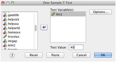
            In this chapter, we discussed methods of testing differences in means between a sample and a population value. SPSS includes a One-Sample T Test procedure to do this test. SPSS does not compute the test with the Z statistic; instead, it uses the t statistic to test for all mean differences. The One-Sample T Test procedure can be found under the Analyze menu choice, then under Compare Means, where it is labeled One-Sample T Test. The opening dialog box (Figure 8.1) requires that you place at least one variable in the Test Variable(s) box. Then a test value must be specified.

            We’ll use the GSS2014-B data set for this demonstration. The standard workweek is thought to be 40 hr, so let’s test to see whether American adults work that many hours each week. In this example, place HRS1 in the Test Variable(s) box and “40” in the Test Value box. Then click on OK to run the procedure.

Figure 8.1. One-Sample T Test Dialog Box

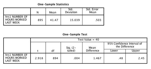
            The output from the One-Sample T Test procedure is not very extensive (see Figure 8.2). A total of 895 people answered the question about number of hours worked per week. The mean number of hours worked is 41.47, with a standard deviation of 15.039. Below this, SPSS lists the test value, 40. It includes the two-tailed significance, or probability, for the one-sample test. This value is .004, given the calculated t statistic of 2.918, with 894 degrees of freedom. Thus, at the .01 significance level, we would reject the null hypothesis and conclude that American adults work more than 40 hr/week.

            SPSS also supplies a 95% confidence interval for the mean difference between the test value and the sample mean. Here, the confidence interval runs from .48 to 2.45, providing estimates of how much more than 40 hr/week Americans work.

Figure 8.2. One-Sample T Test Output

Demonstration 2: Producing a Test of Mean Differences

            In this chapter, we have also discussed methods of testing differences in means or proportions between two samples (or groups). The Two-Sample T Test procedure can be found under the Analyze menu choice, then under Compare Means, where it is labeled Independent-Samples T Test.

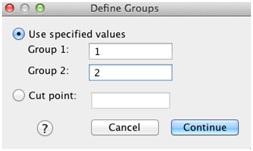
            The opening dialog box requires that you specify various test variables (the dependent variable) and one independent or grouping variable (Figure 8.3). We’ll test the null hypothesis that men and women work the same number of hours each week by using the variable HRS1. Place that variable in the Test Variable(s) box and SEX in the Grouping Variable box. When you do so, question marks appear next to SEX indicating that you must supply two values to define the two groups (independent samples). Click on Define Groups. Then put “1” in the first box and “2” in the second box (1 = male and 2 = female), as shown in Figure 8.4. Then click on Continue and OK to run the procedure.

Figure 8.3. Independent-Samples T Test Dialog Box

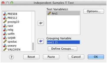
Figure 8.4. Define Groups Dialog Box

            The output from Independent Samples T test (Figure 8.5) is detailed and contains more information than we have reviewed in this chapter. The first part of the output displays the mean number of hours worked for Whites and Blacks, the number of respondents in each group, the standard deviation, and the standard error of the mean. We see that males worked 5.00 hr more per week than females (43.92 – 38.92 = 5.00).

Figure 8.5. Independent-Samples T Test Output

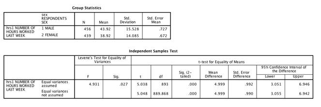
            Earlier in the chapter, we reviewed the Levene’s Test and how to determine whether the variances of the two groups are equal. In this case, we reject the null hypothesis of equal variances (the significance of F is .027 < .05 α). The t obtained is 5.048 (equal variances not assumed) with a probability of .000 (smaller than .05 or .01). We can reject the null hypothesis of no difference and conclude that men work significantly more hours per week than women. The difference of 5.00 hr is significant at the .000 level.

            What if we wanted to do a one-tailed test instead? SPSS does not directly list the probability for a one-tailed test, but it is easy to calculate. If we had specified a directional research hypothesis--such as that men work more hours than women--we would simply take the probability reported by SPSS and divide it into half for a one-tailed test. Because the probability is so large in this case, our conclusion will be the same whether we do a one- or a two-tailed test.

            The last portion of output on each line is the 95% confidence interval for the mean difference in hours worked between the two groups. (Confidence intervals were reviewed in chapter 7.) It is helpful information when testing mean differences because the actual mean difference will vary from sample to sample. The 95% confidence interval gives us a range over which the sample mean differences are likely to vary.

SPSS Problems [GSS14SSDS-B]

1. Use the GSS file to investigate whether or not Americans use the Internet at least 7 hr per week (estimating an hour per day). Perform the One Sample T Test procedure (as presented in SPSS Demonstration 1) to do this test with the variable WWWHR. Do the test at the .01 significance level. What did you find? Do Americans use the Internet 7 hr per week, more or less?

2. The GSS includes a measure of highest educational degree completed (DEGREE). Test whether there is a significant difference between those with less than high school (coded 0) and those with a bachelor’s degree (coded 3) in the number of hours on the Internet per week (WWWHR). Assume α is .05 for a two-tailed test. Summarize your findings.

3. Investigate the difference between individuals who support legalization of marijuana from those who do not based on data from the GSS. Use the variable PRES12 as your independent or grouping variable (1 = Obama and 2 = Romney). Investigate whether there is a significant difference between these two groups in terms of their age (AGE), education (EDUC), and respondent income (NRINCOME06). Assume that α is .05 for a two-tailed test. Based on your analysis, write three Step 5–type statements summarizing your findings.

4. For this analysis, use the variable GOD as your independent variable, comparing individuals who believe in some higher power (3) or know God exists (6). Use the same dependent variables, AGE, EDUC, and NRINCOME06, to estimate t-tests. Assume α is .05 for a two-tailed test. Prepare a statement to summarize your findings.