Do people with more education work more hours per week? Some may argue that those with lower levels of education are forced to work low-paying jobs, thereby requiring them to work more hours per week to make ends meet. Others may rebut this argument by saying those with higher levels of education are in greater positions of authority, which requires more time to ensure operations run smoothly. This question can be explored with SPSS using the techniques discussed in this chapter for interval-ratio data because hours worked last week (HRS1) and number of years of education (EDUC) are both coded at an interval-ratio level in the GSS14SSDS-A file.

 

         We begin by looking at a scatterplot of these two variables. The Scatter procedure can be found under the Graphs menu choice. In the opening dialog box, click Legacy Dialogs then Scatter/Dot (which means we want to produce a standard scatterplot with two variables), select the icon for Simple Scatter, and then click Define.

 

         The Scatterplot dialog box requires that we specify a variable for both the X- and Y-axes. We place EDUC (number of years of education) on the X-axis because we consider it the independent variable and HRS1 (number of hours worked last week) on the Y-axis because it is the dependent variable. Then, click OK.

 

         You can edit it to change its appearance by double-clicking on the chart in the viewer. The action of double-clicking displays the chart in a chart window. You can edit the chart from the menus, from the toolbar, or by double-clicking on the object you want to edit.

 

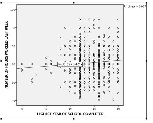
It is difficult to tell whether a relationship exists just by looking at points in the scatterplot, so we will ask SPSS to include the regression line. To add a regression line to the plot, we start by double-clicking on the scatterplot to open the Chart Editor. Click Elements from the main menu, then Fit Line at Total. In the section of the dialog box headed “Fit Method,” select Linear. Click Apply and then Close. Finally, in the Chart Editor, click File and then Close. The result of these actions is shown in Figure 11.1.

 

Figure 11.1. Scatterplot of Hours Worked by Education, Regression Line Plotted

 

         Since the regression line clearly rises as number of years of education increases, we observe the positive relationship between education and number of hours worked last week. The predicted value for those with 20 years of education is about 44 hr, compared with 39.76 hr for those with 10 years of education. However, because there is a lot of scatter around the line (the points are not close to the regression line), the predictive power of the model is weak.

 

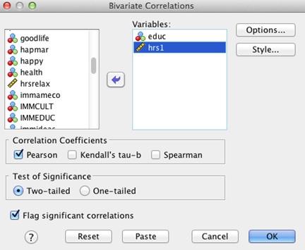
         To further quantify the effect of education on hours worked, we request a correlation coefficient. This statistic is available in the Bivariate procedure, which is located by clicking on Analyze, Correlate, then Bivariate (Figure 11.2). Place the variables you are interested in correlating, EDUC, and HRS1, in the Variable(s) box, then click OK.

 

Figure 11.2. Bivariate Correlations Dialog Box 

         SPSS produces a matrix of correlations, as shown in Figure 11.3. We are interested in the correlation in the bottom left-hand cell, .084. The correlation is significant at the .05 level (two-tailed). We see that this correlation is closer to 0 than to 1, which tells us that education is not a very good predictor of hours worked, even if it is true that those with more education work more hours per week. The number under the correlation coefficient, 895, is the number of valid cases (N)--those respondents who gave a valid response to both questions. The number is reduced.

 

Figure 11.3. Correlation Matrix for Hours Worked and Education

         Next, we will use SPSS to calculate the best-fitting regression line and the coefficient of determination. This procedure is located by clicking on Analyze, Regression, then Linear. The Linear Regression dialog box (Figure 11.4) provides boxes in which to enter the dependent variable, HRS1 and the independent variable, EDUC (regression allows more than one). After you place the variables in their appropriate places, click OK to generate the output. The Linear Regression dialog box offers many other choices, but the default output from the procedure contains all that we need.

 

Figure 11.4. Linear Regression Dialog Box

 

         SPSS produces a great deal of output, which is typical for many of the more advanced statistical procedures in the program. The output is presented in Figure 11.5. Under the Model Summary, the coefficient of determination is labeled “R square.” Its value is .007, which is very weak. Educational attainment explains little of the variation in hours worked, less than 1%.

 

Figure 11.5. Linear Regression Output Specifying the Relationship Between Education and Number of Hours Worked Last Week

         The regression equation coefficients are presented in the Coefficients table. The regression equation coefficients are listed in the column headed “B.” The coefficient for EDUC, or b, is about .417; the intercept term, or a, identified in the “(Constant)” row, is 35.589. Thus, we would predict that every additional year of education increases the number of hours worked each week by about 25 min. Or we could predict that those with a high school level of education work, on average, 35.589 + (.417)(12) hr, or 40.59 hr. 

 

         The ANOVA table provides the results of the analysis of variance test. The table includes regression and residual sum of squares, as well as mean squares. To test the null hypothesis that r² is zero, you will only need the statistic shown in the last column labeled “Sig.” This is the P value associated with the F ratio listed in the column head “F.” The F statistic is 6.368 and its associated P value is .012. This means that there is a little probability (.012) that r² is really zero in the population, given the observed r² of .007. The model, though not reducing much of the variance in predicting work hours, is significant. We are therefore able to reject the null hypothesis at the .05 level.

 

         What other variables, in addition to education, affect the number of hours worked per week? One possible answer to this question is that age (AGE) has something to do with the number of hours worked per week. To answer this question, we will use SPSS to calculate a multiple regression equation and a multiple coefficient of determination. This procedure is similar to the one used to generate the bivariate regression equation. Click Analyze, Regression, then Linear. We place EDUC (number of years of education) and AGE (age in years) in the box for the independent variables and HRS1 (the number of hours worked last week) in the box for the dependent variable, and click OK. The output is presented in Figure 11.6. 

 

         Under the Model Summary, the multiple correlation coefficient labeled “R” is .109. This tells us that education and age are weakly associated with hours worked last week. The coefficient of determination is labeled “R square.” Its value is .012. An R² of .012 means that educational attainment and age jointly explain just 1% of the variation in hours worked last week. In addition, SPSS provides an “Adjusted R square,” which is .01. The “adjusted R square” adjusts the R² coefficient for the number of predictors in the equation. Generally, the adjusted R² will be lower, relative to R², the larger the number of predictors.

 

Figure 11.6. Multiple Regression Output Specifying the Relationship Between Education, Age, and Number of Hours Worked Last Week

         The regression equation coefficients are listed in the Coefficients table. The regression equation coefficients are listed in the column headed “B.” The coefficient for EDUC is about .433, and for AGE, it is –.077. The intercept term, or a, identified in the “(Constant)” row, is 38.815. Thus, we would predict that, holding age constant, every additional year of education increases the number of hours worked the previous week by about 26 min (.43 × 60). 

 

         1. Explore the relationship between the number of siblings a respondent has (SIBS) and his or her number of children (CHILDS).

         2. Use the same variables as in Exercise 1 but do the analysis separately for men and women. Begin by locating the variable SEX. Click Data, Split File, and then select Organize Output by Groups. Insert SEX into the box and click OK. Now, SPSS will split your results by sex.

         3. Use the same variables as in Exercise 1 but do the analysis separately for White and Black respondents. Click Data, Split File, and then select Organize Output by Groups. Insert RACECEN1 into the box and click OK. SPSS will split your results by RACECEN1 (focusing your analysis only on the categories for Whites and Blacks). 

         

         4. Use the same variables as in Exercise 1 but do the analysis separately for married and divorced respondents. Begin by locating the variable MARITAL. Click Data, Split File, and then select Organize Output by Groups. Insert MARITAL into the box and click OK. SPSS will split your results by marital status.

         5. Investigate the relationship between the respondent’s education (EDUC) and the education received by his or her father and mother (PAEDUC and MAEDUC, respectively).