SPSS Exercises
Demonstration 1: Producing Bivariate Tables
SPSS has a separate procedure designed specifically to produce cross-tabulation tables. It is called the Crosstabs procedure and can be found under Descriptive Statistics in the Analyze menu (Analyze, Descriptive Statistics, Crosstabs). The dialog box for Crosstabs requires us to specify both a variable that will define the rows and one that defines the columns of a table. We will investigate the relationship between the importance of being a Christian in order to be truly American (AMCHRSTN) and attitudes toward homosexuality (HOMOSEX). Select AMCHRSTN for the column variable and HOMOSEX for the row variable.
By default, SPSS displays the count in each cell of the table. Click on the Cells button to request percentages (Figure 9.1). As usual, we percentage the table based on the independent or predictor variable, which is religious affiliation. The independent variable is placed in columns, while the dependent variable is placed in rows. We click on the checkbox for “Column” to percentage the table by AMCHRSTN. (Note that “Observed” is already checked by default in the Counts section. In the Noninteger Weights section, “Round cell counts” is checked by default.)
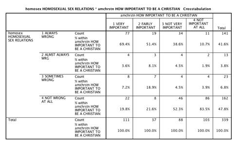
Click on Continue, then OK, to obtain the table shown in Figure 9.2. SPSS displays both the count and the column percentage in each cell. In the upper left corner of the table, the labels “Count” and “% within AMCHRSTN” are displayed as a reminder of what SPSS has placed in each cell. Row totals and column totals are supplied automatically, as is the overall total (339 respondents gave valid responses to both questions).
As you review the table, note how the higher percentages are in opposite corners of the table. In the row for “always wrong” for HOMOSEX--respondents who believe being a Christian is “very important” or “fairly important” are more likely to think homosexual relations is “always wrong” (69% and 51.4%) when compared to those who believe being a Christian is “not very important” (38.6%) or “not important at all” (10.7%). How would you describe the results for the row “not wrong at all” for HOMOSEX? What is the relationship between AMCHRSTN and HOMOSEX?
Figure 9.1. Crosstabs: Cell Display Dialog Box
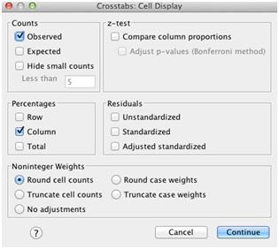
Figure 9.2. Cross-Tabulation Output: AMCHRSTN and HOMOSEX
Demonstration 2: Producing Tables With a Control Variable
As we’ve seen in this chapter, the analysis of data is enhanced when a third variable--a control variable--is added to a bivariate table. In the Crosstabs procedure, the third variable is added in the Layer section of the main dialog box (Figure 9.3). (This box is labeled “Layer 1 of 1” because it is possible to have additional levels of control, which are accessed by clicking on the Next button.) We will not change HOMOSEX and AMCHRSTN but will add SEX as the control variable. There is no need to change the numbers displayed in the cells: The observed count and column percentages are still correct choices. Figure 9.4 shows the bivariate tables for men and women separately.
Figure 9.3. Crosstabs Dialog Box
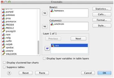
Figure 9.4. Cross-Tabulation Output: AMCHRSTN by HOMOSEX Controlling for SEX
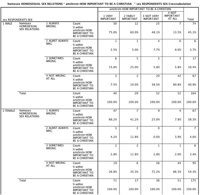
The relationship we observed in the original table (Figure 9.2) is present in this analysis--if respondents believe being a Christian is important to being an American, they are more likely to indicate that homosexuality is always wrong. But when controlling for sex, note how most men believe that homosexuality is “always wrong” (three of the four AMCHRSTN modes--75%, 60%, and 48.1%--are in the HOMOSEX category “always wrong”). In contrast, for women, the AMCHRSTN modes are split into two HOMOSEX categories--always wrong (66.2% and 41.2%) and not wrong at all (72.2% and 86.3%). The relationship between AMCHRSTN and HOMOSEX appears to be slightly stronger for women. In the next chapter, we will use the Statistics button in the Crosstabs dialog box to request additional output to further interpret and evaluate bivariate tables.
For Demonstrations 3 and 4, Switch to the [GSS14SSDS-A] Data Set
Demonstration 3: Producing the χ2 Statistic for Cross-Tabulations
The SPSS Crosstabs procedure can also be used to calculate a χ2 value for a bivariate table.
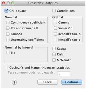
Click on Analyze, Descriptive Statistics, and Crosstabs, then on the Statistics button. You will see the Dialog box shown in Figure 9.5. To request the χ2 statistic, click on the Chi-square box in the upper left corner. You can also request expected frequencies via the Cells button.
Figure 9.5. Crosstabs Statistics Dialog Box
Click on Continue. In this demonstration, we will look at the relationship between educational degree (DEGREE) and political views (POLVIEWS). Place POLVIEWS in the Row(s) box and DEGREE in the Column(s) box. Then, click on OK to run the procedure.
The resulting output includes the χ2 statistics as shown in Figure 9.6. SPSS produces quite a bit of output, perhaps more than what is expected. We will concentrate on the first row of information, Pearson’s χ2.
Pearson’s χ2 has a value of 53.733 with 24 degrees of freedom. SPSS calculates the significance of this χ2 to be .000. Educational degree and political views are related. Specifically, as educational degree increases (graduate degree attainment), it appears that men and women are more likely to report being “extremely liberal.”
Figure 9.6. χ2 Test Output for DEGREE by POLVIEWS
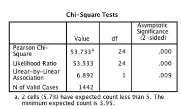
The last portion of the output from SPSS allows us to check for the assumption that all expected values in each cell of the table are 5 or greater. The output indicates that two of the cells or 5.7% have a value less than 5. This is lower than our threshold of 20%.
Demonstration 4: Producing Nominal and Ordinal Measures of Association for Bivariate Tables
The SPSS Crosstabs procedure can also be used to calculate measures of association. We’ll begin by investigating the relationship between belief in the Bible (BIBLE) and support for legal abortions for women for any reason (ABANY).
Click on Analyze, Descriptive Statistics, then Crosstabs to get to the Crosstabs dialog box. Put ABANY in the Row(s) box and BIBLE in the Column(s) box. Then click on the Statistics button. The Statistics dialog box (Figure 9.5) has about a dozen statistics from which to choose. Note that four statistics are listed in separate categories for “Nominal” and “Ordinal” data. λ is listed in the former, and γ and Kendall’s τ-b in the latter. Cramer’s V can be easily obtained by checking the Phi and Cramer’s V box. The other measures of association, such as Somer’s d and φ, will not be discussed in this textbook.
Since both variables are nominal, check the box for λ. It is critical that we, as users of statistical programs, understand which statistics to select in any procedure. SPSS, like most programs, can’t help us select the appropriate statistic for an analysis. Now click on Continue and then OK to create the table.
The first table is Case Processing Summary showing the number of valid and missing cases (not shown here). The second table should be a bivariate table of our two variables (not shown). Below is a table labeled “Directional Measures” (Figure 9.7). For now, we will only concern ourselves with the first two columns. λ is listed with three values. We’ve learned that the value of λ depends on which variable is considered the dependent variable. In our example, attitude toward abortion for any reason is dependent, so λ is .216. This indicates a weak relationship between the two variables. We can conclude that knowing the respondent’s belief about the Bible increases the ability to predict his or her abortion attitude by just 21.6%.
SPSS also calculates a symmetrical λ for those tables, where there is no independent or dependent variable. This calculation goes beyond the scope of this book. In addition, SPSS provides the Goodman and Kruskal statistic, another nominal measure of association, even though it was not requested. These measures will always be produced when λ is requested.
If we checked for the φ and Cramer’s V in the Statistics dialog box, the Symmetric Measures table should be included in the output (Figure 9.7).
Figure 9.7. Measures of Association for BIBLE and ABANY
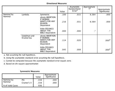
Cramer’s V is .338, which indicates a moderate association between belief in the Bible and support for legal abortions for women for any reason.
We can also use the same procedures to calculate γ for ordinal measures. For this demonstration, we’ll examine the relationship between educational attainment (DEGREE) and attitudes toward same-sex marriage (MARHOMO). Respondents were asked whether homosexuals should have the right to marry (strongly agree, agree, neither, disagree, strongly disagree). Both variables are ordinal measurements.
Click on Analyze, Descriptive Statistics, then Crosstabs to get to the Crosstabs dialog box. Put MARHOMO in the Row(s) box and DEGREE in the Column(s) box. Then click on the Statistics button. The Statistics dialog box has about a dozen statistics from which to choose. Click on γ and Kendall’s τ-b listed in the ordinal box. SPSS produces two separate tables (other than Case Processing Summary), the first is the bivariate table between MARHOMO and DEGREE and the second is the table of symmetric measures, γ and Kendall’s τ-b, which we requested (Figure 9.8).
Figure 9.8. SPSS Output Displaying the Relationship Between DEGREE and MARHOMO

The Kendall’s τ-b statistic is in the first row under the column labeled “Value” followed by the γ statistic. For this bivariate table, both the Kendall’s τ-b statistic (–.219) and the γ statistic (–.299) indicate a weak negative relationship between educational level and attitudes toward same-sex marriage. Using Kendall’s τ-b, we can reduce about 22% of our error in predicting attitudes toward same-sex marriage by using information about respondent’s education. Using γ, about 30% of the error in predicting attitudes toward same-sex marriage would be reduced if we had information about respondent’s educational attainment. Note that given how MARHOMO is coded, the negative γ indicates that as DEGREE increases, respondents are more likely to strongly agree/agree that homosexuals should have the right to marry.
SPSS Problems [GSS14SSDS-B]
1. The GSS data set includes responses to questions about the respondent’s homeownership status (DWELOWN) and his or her subjective class identification (CLASS). Analyze the relationship between responses to these two questions with the SPSS Crosstabs procedure, requesting counts and appropriate cell percentages. (Click on Analyze, Descriptive Statistics, and Crosstabs to get started.)
a. What percentage of the working-class group responded that they “pay rent?”
b. What percentage of the lower-class group were homeowners?
c. What percentage of those who were homeowners were also from the middle and upper classes?
d. Is there a relationship between perceived class and homeownership? If there is a relationship, describe it.
e. Rerun your analysis, this time adding RACE as a control variable. Is there a difference in the relationship between perceived class and homeownership for Whites and Blacks?
2. GSS respondents were asked to report which candidate they voted for in the 2012 presidential election (PRES12). Examine the relationship between PRES12, CLASS, and SEX. Use SEX as the control variable. Does presidential voting vary by one’s social class and sex? Explain.
3. In this exercise, we test the relationship between 2008 and 2012 presidential election voting (PRES08 and PRES12) and respondent’s feelings about the Bible (BIBLE).
a. Which variable should be defined as the dependent variable? Explain your answer.
b. Using SPSS Crosstabs, create two tables with BIBLE and each of the PRES variables. Explain the relationship between the two variables for 2008 and 2012. (When you discuss your findings, exclude those respondents who did not vote.) If the respondent believes the Bible is the word of God, how did the respondent vote in 2008 or 2012?
c. Examine the relationship between BIBLE and one of the PRES variables with a control variable of your choice.
4. Describe the relationship between PRES12 and agreement to the statement, “America should exclude illegal immigrants” (EXCLDIMM). Define PRES12 as the dependent variable.
For Exercises 5–9, Switch to the [GSS14SSDS-A] Data Set
5. Does marital happiness vary by respondent’s sex?
a. Use SPSS to investigate the relationship between SEX and HAPMAR (happiness of marriage). Create a bivariate table and ask for appropriate percentages and expected values. Does the table have a large number of cells with expected values less than 5? Are there any surprises in the data?
b. Have SPSS calculate χ2 for the table.
c. Test the null hypothesis at the .05 significance level. What do you conclude?
d. Select another demographic variable (DEGREE or CLASS) and investigate its relationship with HAPMAR.
6. Investigate the relationship between social class (CLASS) and general happiness rating (HAPPY). Does money buy happiness? Have SPSS calculate the cross-tabulation, along with χ2 (set α at .05). What can you conclude?
7. Examine the relationships between respondent’s health (HEALTH) and educational degree (DEGREE). Define DEGREE as your independent variable.
a. Request the appropriate measures of association to describe the relationship between these two variables. Interpret your measures of association.
b. Calculate the χ2 for the table. Test the null hypothesis at the .05 level. What do you conclude?
8. Reexamine the relationship between the importance of being a Christian in order to be truly American (AMCHRSTN) and attitudes toward homosexuality (HOMOSEX) which we first explored in chapter 9’s SPSS Demonstration. Use the GSS14SSDS-B data set.
a. Which variable is the dependent variable? Explain.
b. Identify and calculate the appropriate measure of association to describe the relationship between the two variables.
c. Add SEX as a control variable and calculate the γ for each partial table. Is the relationship stronger for women or men? Can you think of reasons why this might be so?
9. Investigate the relationship between the abortion attitudes in GSS14SSDS-A (e.g., ABANY, ABMORE, ABSINGLE, and ABPOOR) and various demographic variables (you might begin with gender, age, or race). Examine the relationship of these variables based on the appropriate measures of association. For example, you might examine whether attitude toward each of the abortion items has a similar relationship to gender. That is, if females are supportive of abortion for rape victims, are they also supportive of abortion in other circumstances? Try exploring these relationships further by adding control variables. You might create tables of abortion attitude by race and by gender. When you have finished the analysis, write a short report summarizing the findings. Suggest possible causes for the relationships you found.
