Demonstration 1: Producing Measures of Variability With Frequencies

            Except for the IQV, the SPSS Frequencies procedure can produce all the measures of variability we’ve reviewed in this chapter. (SPSS can be programmed to calculate the IQV, but the programming procedures are beyond the scope of our book.)

            We’ll begin with Frequencies and calculate various statistics for AGE. If we click on Analyze, Descriptive Statistics, Frequencies, then on the Statistics button, we can select the appropriate measures of variability.

            The measures of variability available are listed in the Dispersion box at the bottom of the dialog box. We’ve selected the standard deviation, variance, and range, plus the mean and median (in the Central Tendency box) for reference. In the Percentile Values box, we’ve selected Quartiles to tell SPSS to calculate the values for the 25th, 50th, and 75th percentiles. SPSS also allows us to specify exact percentiles in this section (such as the 34th percentile) by typing a number in the box after “Percentile(s)” and then clicking on the Add button.

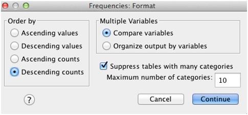
            Earlier, we had seen the frequency table for the variable AGE, so after clicking on Continue, we click on Format to turn off the display table. This is done by clicking on the button for “Suppress tables with many categories” (see Figure 4.1). There are other formatting options here that you may explore later when using SPSS.

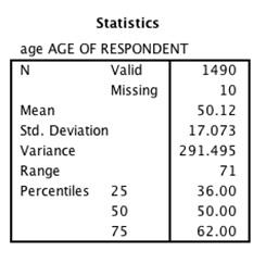
            Click on Continue, then OK to run the procedure. SPSS produces the mean and the other statistics we requested (Figure 4.2). The range of age is 71 years (from 18 to 89). The standard deviation is 17.073, which indicates that there is a moderate amount of dispersion in the ages. The variance, 291.495, is the square of the standard deviation (17.073).

            The value of the 25th percentile is 36, the value of the 50th percentile (which is also the median) is 50, and the value of the 75th percentile is 62. Although Frequencies does not calculate the IQR, it can easily be calculated by subtracting the value of the 25th percentile from the 75th percentile, which yields a value of 26 years. Compare this value with the standard deviation.

Figure 4.1. Format Dialog Box

Figure 4.2. Descriptive Statistics for AGE

Demonstration 2: Producing Measures of Variability With Explore

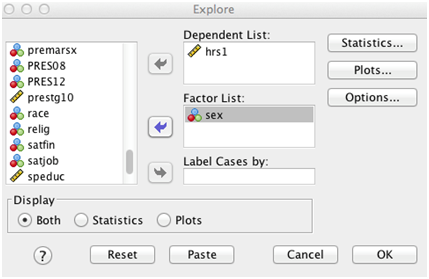
            Another SPSS procedure that can produce the usual measures of variability is Explore. The Explore procedure is located in the Descriptive Statistics section of the Analyze menu. In its main dialog box (Figure 4.3), the variables for which you want statistics are placed in the Dependent List box. You have the option of putting one or more nominal variables in the Factor List box; Explore will display separate statistics for each category of the nominal variable(s) you’ve selected.

Figure 4.3. Explore Dialog Box

            Place the variable HRS1 (number of hours worked last week) in the Dependent box and SEX in the Factor box to provide separate output for males and females. Click OK. By default, Explore will produce statistics and plots, so we don’t need to make any other choices. Although our request will not produce percentiles or create a histogram, Explore has options to do both plus several other tasks.

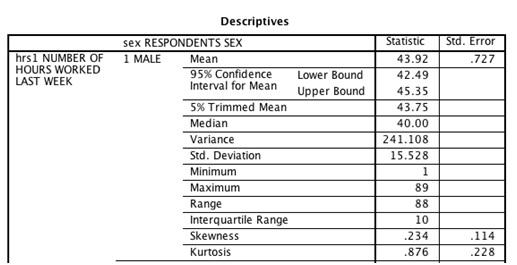
            Selected output for males is shown in Figure 4.4. Though not replicated here, you’ll notice that the first table is the Case Processing Summary Table. It indicates that 456 males answered this question. The valid sample of females is also reported, 439. Based on the second table, Descriptives, we know that for males, the mean number of hours worked last week is 43.92; the median is 40.00. The standard deviation is 15.528, the range is 88, and the IQR is 10, which is quite narrow compared with the range. (A stem-and-leaf plot--another way to visually present and review data--is also displayed by default. However, we will not cover stem-and-leaf plots in this textbook. The option for the stem-and-leaf plot can be changed so that it will not be displayed.)

Figure 4.4. Descriptive Statistics for HRS1, Men Only

            Although not displayed here, the mean number of hours worked last week for females is 38.92; the median is 40. The standard deviation is 14.085, the IQR is 13, and the range is 88--values somewhat smaller than those for males with the exception of the range and the IQR. The variation in the number of hours worked last week is also slightly smaller for females than those for males.

SPSS Problems [GSS14SSDS-B]

1. Use the Frequencies procedure to investigate the variability of the respondent’s current age (AGE). Click on Analyze, Descriptive Statistics, Frequencies, and then Statistics. Select the appropriate measures of variability. How would you describe the distribution of AGE?

2. Using the Explore procedure, separate the statistics for EDUC (education) and PRESTG10 (occupational prestige score) for men and women, selecting SEX as a factor variable in the Explore window. Click on Analyze, Descriptive Statistics, Explore, and then insert EDUC and PRESTG10 into the Dependent List and SEX in the Factor List. What differences exist in the educational attainment and occupational prestige of men and women? Assess the differences between men and women based on measures of central tendency and variability.

3. Repeat the procedure in Exercise 2, investigating the dispersion in NRINCOME06 (recoded income). Select your own factor (nominal) variable to make the comparison (such as CLASS, RACE, or some other factor). Click on Analyze, Descriptive Statistics, Explore, and insert NRINCOME06 into the Dependent List and your factor variable of choice in the Factor List. In a paragraph or two, use appropriate measures of variability to summarize the results.

4. Examine the number of hours that Blacks and Whites work each week. The variable HRS1 measures the number of hours a respondent worked the week before the interview. Use the Explore procedure to study the variability of hours worked, comparing Blacks and Whites (RACE) in the GSS sample. Is there a difference between the two groups in the variability of work hours?