The variance measures the fit of the mean, or the average error between the mean and the observed scores.

The variance in the sample will underestimate the variance in the population because the sample is likely to be narrower than the population from which it comes. This is because scores at the extremes of the population occur less often and so are less likely to appear in the sample.

It tells us that most of the scores cluster close to the mean and so the mean is a good ‘fit’ to the data.

To compute the mean, we use the equation:

To calculate the median, we first arrange the scores in ascending order: 7, 9, 16, 20, 21, 26, 28, 32, 45. Next, we find the position of the middle score by counting the number of scores we have collected (n), adding 1 to this value, and then dividing by 2. With 9 scores, this gives us (n + 1)/2 = (9 + 1)/2 = 10/2 = 5. Then we find the score that is positioned at the location we have just calculated. So in this example we find the 5th score, which is 21. Therefore, the median is 21.

The mode is the most frequent score. However, in this dataset all the scores are different so there is no mode.

First we need to compute the mean:

To calculate the sum of squares, subtract the mean from each score, then square each deviance. Finally, add up these squared deviances (Table 1).

Table 1: Calculating the sum of squared errors

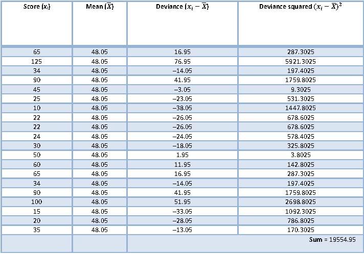
So, the sum of squared errors is a massive 19,554.95.

The variance is the sum of squared errors divided by the degrees of freedom (N - 1). There were 20 scores and so the degrees of freedom were 19. The variance is, therefore, 19,554.95/19 = 1029.21.

The standard deviation is the square root of the variance:  = 32.08.

The standard deviation in puzzle 5 was 32.08 and the mean was 48.05. This is a huge standard deviation relative to the mean: over half its size! This suggests that the data points are distant from the mean and so the mean is not a good ‘fit’ to the data.

First we need to compute the mean:

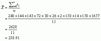
Then we compute the standard deviation starting with the sum of squared errors, which is 2,268,540.91 (Table 2).

Table 2: Calculating the sum of squared errors

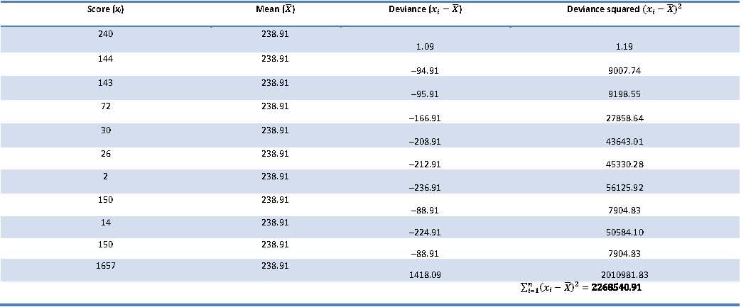
We use the sum of squares to calculate the variance:

We can now calculate the standard deviation:

days

To calculate the median, range and interquartile range, first arrange the scores in ascending order: 2, 14, 26, 30, 72, 143, 144, 150, 150, 240, 1657.

The median: The median will be the score in position (n + 1)/2. There are 11 scores, so this will be the 12/2 = 6th score. The 6th score in our ordered list is 143. The median length of these celebrity marriages is therefore 143 days.

The lower quartile: This is the median of the lower half of scores. If we split the data at 143 (the 6th score), there are 5 scores below this value. The median of these 5 will be the 6/2 = 3rd score. The 3rd score is 26. The lower quartile is therefore 26 days.

The upper quartile: This is the median of the upper half of scores. If we split the data at 143 again (not including this score), there are 5 scores above this value. The median of these 5 will be the 6/2 = 3rd score above the median. The 3rd score above the median is 150; the upper quartile is therefore 150 days.

The range: This is the highest score (1657) minus the lowest (2), i.e., 1655 days.

The interquartile range: This is the difference between the upper and lower quartile: 150 − 26 = 124 days.

First let’s compute the new mean:

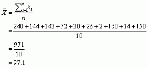
The mean length of celebrity marriages is now 97.1 days, compared to 238.91 days when Jennifer Aniston and Brad Pitt’s marriage was included. This demonstrates that the mean is greatly influenced by extreme scores.

Let’s now calculate the standard deviation excluding Jennifer Aniston and Brad Pitt’s marriage, starting with the sum of squared errors, which is 56,460.9 (Table 3).

Table 3: Calculating the sum of squared errors

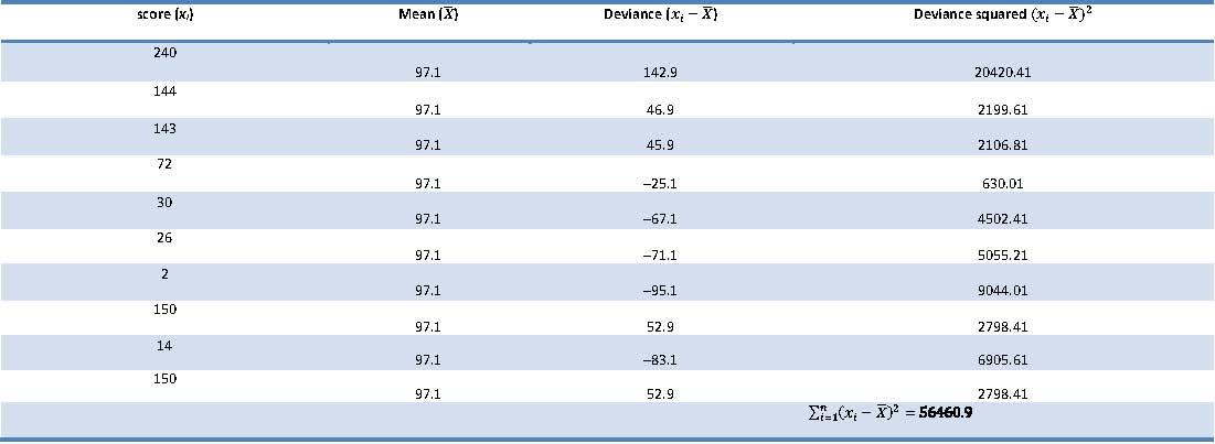
The variance is

We can now calculate the standard deviation:

From these calculations we can see that the variance and standard deviation, like the mean, are both greatly influenced by extreme scores. When Jennifer Aniston and Brad Pitt’s marriage was included in the calculations (see puzzle 7), the variance and standard deviation were much larger: 22,6854.09 and 476.29, respectively. Therefore, by removing the outlier (Jen and Brad’s marriage) the mean is now a better ‘fit’ to the data.

To calculate the median, range and interquartile range, first, arrange the scores in ascending order but this time excluding Jennifer Aniston and Brad Pitt’s marriage:

2, 14, 26, 30, 72, 143, 144, 150, 150, 240.

The median: The median will be score in position (n + 1)/2. There are now 10 scores, so this will be the 11/2 = 5.5th. Therefore, we take the average of the 5th score and the 6th score. The 5th score is 72, and the 6th is 143; the median is therefore 107.5 days. Like the mean, the median has reduced because the extreme score has been omitted; however, the reduction is less dramatic than it was for the mean, showing how the median is relatively less affected by extreme scores than the mean.

The lower quartile: This is the median of the lower half of scores. If we split the data at 107.5 (this score is not actually present in the data set), there are 5 scores below this value. The median of these 5 will be the 6/2 = 3rd score. The 3rd score is 26; the lower quartile is therefore 26 days.

The upper quartile: This is the median of the upper half of scores. If we split the data at 107.5 (this score is not actually present in the data set), there are 5 scores above this value. The median of these 5 will be the 6/2 = 3rd score above the median. The 3rd score above the median is 150; the upper quartile is therefore 150 days.

The range: This is the highest score (240) minus the lowest (2), i.e., 238 days. You’ll notice that without the extreme score the range drops dramatically from 1655 to 238 – around a seventh of the size.

The interquartile range: This is the difference between the upper and lower quartile: 150 − 26 = 124 days of marriage. This is the same as the value we got when Jennifer Aniston and Brad Pitt’s marriage was included. This demonstrates the advantage of the interquartile range over the range: it isn’t affected by extreme scores at either end of the distribution.

First we need to compute the mean:

Then the standard deviation starting with the sum of squared errors, which is 83.73 (Table 4).

Table 4: Calculating the sum of squared errors

So, the sum of squared errors is 83.73. To calculate the variance, we divide this value by the degrees of freedom (N-1):

We can now calculate the standard deviation as the square root of this value:

To calculate the median, range and interquartile range, first arrange the scores in ascending order: 2, 3, 4, 5, 5, 5, 6, 7, 7, 8, 8, 8, 9, 10, 10.

The median: The median will be the score in position (n + 1)/2. There are 15 scores, so this will be the 16/2 = 8th score, which in our ordered list is 7.

The lower quartile: This is the median of the lower half of scores. If we split the data at 7 (the 8th score), there are 7 scores below this value. The median of these 7 will be the 8/2 = 4th score. The 4th score is 5. The lower quartile is therefore 5.

The upper quartile: This is the median of the upper half of scores. If we split the data at the 8th score again, there are 7 scores above this value. The median of these 7 will be the 8/2 = 4th score above the median. The 4th score above the median is 8; the upper quartile is therefore 8.

The range: This is the highest score (10) minus the lowest (2), i.e., 8.

The interquartile range: This is the difference between the upper and lower quartile: 8 − 5 = 3.

The mean in puzzle 9 was 6.47 and the standard deviation was 2.45. A standard deviation of 2.45 is very large relative to a mean of 6.47, suggesting that the mean is not a particularly good ‘fit’ to the data.