An Adventure in Statistics: The Reality Enigma
Student Resources
Jig:Saw’s puzzle solutions
Puzzle 1
Explain the central limit theorem.
This theorem states that when samples are large (above about 30) the sampling distribution will take the shape of a normal distribution regardless of the shape of the population from which the sample was drawn. For small samples, the t-distribution better approximates the shape of the sampling distribution. We also know from this theorem that the standard deviation of the sampling distribution (i.e., the standard error of the sample mean) is well approximated by the standard deviation of the sample(s) divided by the square root of the sample size (N).
Puzzle 2
Using the data in Table 8.2 (in the book and reproduced below), what was the mean accuracy in both the fake-name group and the own-name group?
To calculate the mean accuracy in both groups, we need to add together all the scores in each group and then divide the sum by the total number of scores. If we start with the own-name group, the sum of all the scores added together was 1547 and there were 35 scores in total, so the mean accuracy in the own-name group was 1547/35 = 44.2. In the fake-name group, the sum of all the scores was 1806 and there were 33 scores in total, so the mean accuracy in the fake-name group was 1806/33 = 54.73.
Table 8.2 (reproduced): Female participants’ accuracy on a maths test grouped by whether they took the test under their own or a fake name (a subset of the data from Zhang et al.)

Puzzle 3
Using the data in Table 8.2 (in the book and reproduced above), what was the standard error in both the fake-name group and the own-name group?
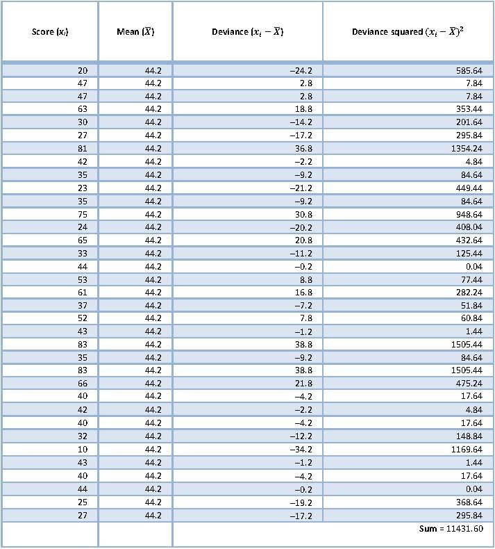
Let’s start with the own-name group. First we need to calculate the sum of squares by subtracting the mean from each score, squaring each deviance and then adding up the squared deviances (Table 1).
Table 1: Calculating the sum of squares for the own-name group

So, the sum of squared errors is 11,431.6. The variance is the sum of squared errors divided by the degrees of freedom (N - 1). There were 35 scores and so the degrees of freedom were 34. The variance is, therefore, 11,431.6/34 = 336.22.
The standard deviation is the square root of the variance: ![]() = 18.34.
= 18.34.
We can now calculate the standard error using equation (8.3) in the book, ![]() , which states that the standard error of the mean is the sample standard deviation divided by the square root of the sample size.
, which states that the standard error of the mean is the sample standard deviation divided by the square root of the sample size.
![]()
So, the standard error of the own-name group is 3.10.
Now let’s calculate the standard error of the fake-name group in exactly the same way as we did for the own-name group.
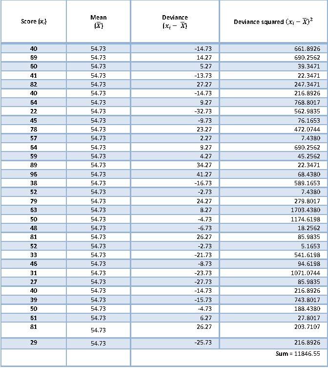
Table 2: Calculating the sum of squares for the fake-name group

The sum of squared errors is 11,846.55 and the variance is the sum of squared errors divided by the degrees of freedom (N - 1). There were 33 scores and so the degrees of freedom were 32. The variance is, therefore, 11,846.55/32 = 370.20.
The standard deviation is the square root of the variance: ![]() = 19.24.
= 19.24.
We can calculate the standard error in the same way as for the own-name group (see above):
![]()
The standard error of the fake-name group is, therefore, 3.35.
Puzzle 4
What is a 95% confidence interval?
For a given statistic (e.g., the mean) calculated for a sample of observations, a 95% confidence interval is a range of values around that statistic that are believed to contain the true value of that statistic (i.e., the population value) in 95% of samples. It’s worth remembering that for a particular sample you can’t be sure whether it is one of the 95% for which the interval contains the population value or whether it is one of the 5% that does not.
Puzzle 5
Using the data in Table 8.2 (in the book and reproduced in puzzle 2), calculate the 95% confidence interval for the mean in both the fake-name group and the own-name group.
We have already calculated the mean and standard error for both groups (see puzzles 2 and 3), so all we need to do is to plug these values into the following equations:
![]()
![]()
For the own-name group:
![]()
![]()
For the fake-name group:
![]()
![]()
Puzzle 6
Using the 95% confidence intervals for the own-name and fake-name groups, can you infer anything about whether the accuracy on the maths test was affected by whether the test was taken under their own or a fake name?
The 95% confidence interval for the fake-name group ranged from 48.16 to 61.30, and for the own-name group it ranged from 38.12 to 50.28. Therefore, the intervals overlap, but only just: the upper limit of the own-name group (50.28) is only slightly larger than the lower limit of the fake-name group (48.16). If we assume that both samples are ones from the 95% that produce intervals that contain the population value, then what this implies is that the population values for ‘own name’ and ‘fake name’ are very unlikely to be the same (because the intervals barely overlap). We might infer from this that the mean accuracy on the maths test was genuinely higher when taken under a fake name than when taken under their own name.
Puzzle 7
Using the data in Table 8.2 (in the book and reproduced in puzzle 2), calculate the 99% confidence interval for the mean in both the fake-name group and the own-name group.
![]()
![]()
For the own-name group:
![]()
![]()
For the fake-name group:
![]()
![]()
Puzzle 8
Using the data in Table 8.2 (in the book and reproduced in puzzle 2), calculate the 95% confidence interval for the first 10 scores in the fake-name group.
First we need to calculate the mean of the first 10 scores:
![]()
Then we need to calculate the sum of squares by subtracting the mean from each score, squaring each deviance and then adding up the squared deviances (Table 3).
Table 3: Calculating the sum of squares for the first 10 scores of the fake-name group

So, the sum of squared errors was 3386.9. The variance is the sum of squared errors divided by the degrees of freedom (N - 1). There were 10 scores and so the degrees of freedom were 9. The variance is, therefore, 3386.9/9 = 376.32.
The standard deviation is the square root of the variance: ![]() = 19.40.
= 19.40.
We can now calculate the standard error using equation (8.3) in the book, ![]() , which states that the standard error of the mean is the sample standard deviation divided by the square root of the sample size.
, which states that the standard error of the mean is the sample standard deviation divided by the square root of the sample size.
![]()
So the standard error of the first 10 scores in the fake-name group was 6.13.
We can now calculate the 95% confidence interval, but because we have a small sample size (less than 30), instead of using the value of z from a normal distribution, we use the value of t from the t-distribution appropriate for our sample size by using equation (8.8) in the book:
![]()
![]()
First, if n = 10, then the degrees of freedom will n-1 = 10-1 = 9. The corresponding value of t (df = 9) for a 95% CI is 2.262. This gives us the following limits:
![]()
![]()
Puzzle 9
What is a sampling distribution?
We can think of a sampling distribution like this: if we took a sample from a population and calculated a statistic (e.g., the mean), the value of this statistic would depend somewhat on the sample we took. As such the statistic will vary slightly from sample to sample. If, hypothetically, we took lots and lots of samples from the population and calculated the statistic of interest, we could create a frequency distribution of the values we got. The resulting distribution is what the sampling distribution represents: the distribution of possible values of a given statistic that we could expect to get from a given population.
Puzzle 10
What is the difference between the standard error of the mean and the standard deviation?
The standard deviation measures how representative the mean is of the observed data. A small standard deviation (relative to the value of the mean) indicates that data points are close to the mean. A large standard deviation (relative to the mean) indicates that the data points are distant from the mean. In contrast, the standard error of the mean is the standard deviation of sample means. As such, it is a measure of how representative a sample mean is likely to be of the population mean. A large standard error (relative to the sample mean) indicates that there is a lot of variability between the means of different samples and so the sample might not be representative of the population. A small standard error indicates that most sample means are similar to the population mean and so our sample is likely to be an accurate reflection of the population.
