An Adventure in Statistics: The Reality Enigma
Student Resources
Jig:Saw’s puzzle solutions
Puzzle 1
Table 13.7 (in the book, reproduced below) shows the infidelity data from the Mark et al. (2011) study but for women. Compute the chi-square statistic and standardized residuals for these data
Table 13.7 (reproduced): Contingency table showing how many women engaged in infidelity or not, based on how happy they were in their relationship. Data from Table 3 of Mark et al. (2011)

First we need to calculate the expected values for each cell in Table 13.7.
![]()
![]()
![]()
![]()
I have tabulated these expected values in Table 1.
Table 1: Contingency table showing the predicted values from the model for each cell in Table 13.7

To compute the chi-square statistic we take each value in each cell of Table 13.7, subtract from it the corresponding model value in Table 1, square the result, and then divide by the corresponding model value. Once we’ve done this for each cell in the table, we add them up:
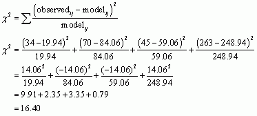
The degrees of freedom are calculated as (r − 1)(c − 1), in which r is the number of rows and c is the number of columns; in other words it is the number of levels of each variable minus one multiplied. In this case the df will be (2 − 1)(2 − 1) = 1. We now need to look up the critical values for the chi-square distribution with df = 1 (Section A.3 of the book), and we will see that they are 3.84 (p = 0.05) and 6.63 (p = 0.01). Because the chi-square value that we calculated is bigger than these values it means that the probability of getting a value at least as big as 16.4 if there were no association between the variables in the population is less than 0.01. With a computer we’d be able to work out the exact value of the probability. In any case, the probability is small enough that we might reject the possibility that infidelity and relationship happiness are not related at all in women.
The puzzle also asks us to calculate the standardized residuals for these data (tabulated in Table 2):
![]()
![]()
![]()
![]()
Table 2: Contingency table showing the standardized residuals for each cell in Table 13.7

Puzzle 2
Table 13.8 (in the book and reproduced below) shows the number of women who were unfaithful or not, based on whether they felt sexually compatible with their partner (data from Mark et al., 2011). Compute the chi-square statistic and standardized residuals for these data.
Table 13.8 (reproduced): Contingency table showing how many women engaged in infidelity or not, based on how compatible they felt with their partner. Data from Table 3 of Mark et al. (2011)

First we need to calculate the expected values for each cell in Table 13.8.
![]()
![]()
![]()
![]()
I have tabulated these expected values in Table 3.
Table 3: Contingency table showing the predicted values from the model for each cell in Table 13.8

To compute the chi-square statistics we take each value in each cell of Table 13.8, subtract from it the corresponding model value in Table 3, square the result, and then divide by the corresponding model value. Once we’ve done this for each cell in the table, we add them up:
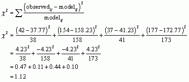
The degrees of freedom will be the same as in the previous puzzle, df = (2 − 1)(2 − 1) = 1; therefore, the critical values for the chi-square distribution will again be 3.84 (p = 0.05) and 6.63 (p = 0.01). Because the chi-square value that we calculated is smaller than these values it means that the probability of getting a value at least as big as 1.12 if there were no association between the variables in the population is greater than 0.05. With a computer we’d be able to work out the exact value of the probability. In any case, because the probability is larger than the critical value of 0.05, it suggests that for women, infidelity and compatibility are not significantly related. The puzzle also asks us to calculate the standardized residuals for these data (tabulated in Table 4):
![]()
![]()
![]()
![]()
Table 4: Contingency table showing the standardized residuals for each cell in Table 13.8

Puzzle 3
Table 13.9 (in the book and reproduced below) shows the number of men who were unfaithful or not, based on whether they felt sexually compatible with their partner (data from Mark et al., 2011). Compute the chi-square statistic and standardized residuals for these data.
Table 13.9 (reproduced): Contingency table showing how many men engaged in infidelity or not based on how compatible they felt with their partner. Data from Table 3 of Mark et al. (2011)

First we need to calculate the expected values for each cell in Table 13.9.
![]()
![]()
![]()
![]()
I have tabulated these expected values in Table 5.
Table 5: Contingency table showing the predicted values from the model for each cell in Table 13.9

To compute the chi-square statistics we take each value in each cell of Table 13.9 (the observed values) subtract from it the corresponding model value in Table 5 (the predicted values) square the result, and then divide by the corresponding model value (or predicted value). Once we’ve done this for each cell in the table, we add them up:
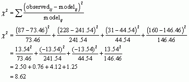
The degrees of freedom will be the same as in the previous two puzzles, df = (2 − 1)(2 − 1) = 1. Therefore, the critical values for the chi-square distribution will again be 3.84 (p = .05) and 6.63 (p = .01). Because the chi-square value that we calculated is larger than these values (8.62) it means that the probability of getting a value at least as big as 8.62 if there were no association between the variables in the population is less than 0.01. With a computer we’d be able to work out the exact value of the probability. In any case, the probability is small enough that we might reject the possibility that infidelity and compatibility are not related at all in men. The puzzle also asks us to calculate the standardized residuals for these data (tabulated in Table 6):
![]()
![]()
![]()
![]()
Table 6: Contingency table showing the standardized residuals for each cell in Table 13.9

Puzzle 4
For puzzles 1-3 calculate the chi-square test using Yates’s correction.
Yates’s continuity correction adjusts the formula for the chi-square statistic slightly so that you subtract 0.5 from the absolute value of the difference between observed and expected frequencies before you square the difference:

For puzzle 1:

The chi-square value using Yates’s correction is 15.26, which is lower than 16.40 - the value when the correction wasn’t applied. The fact that the test statistic has got smaller means that the exact p-value will be smaller too. The correction makes the test stricter.
For puzzle 2:

The chi-square value using Yates’s correction for puzzle 2 is 0.88, which is even lower than 1.12- the value when the correction wasn’t applied.
For puzzle 3:

The chi-square value using Yates’s correction for puzzle 3 is 8.00, which is a fair bit lower than 11.52 - the value when the correction wasn’t applied.
Puzzle 5
For puzzles 1-3 calculate the likelihood ratio.
For each puzzle we can use this equation. The observed values come from the tables of original observations, and the model values come from the tables of expected values that we calculated in each puzzle.
![]()
For puzzle 1:
We use the values in Table 13.7 for the observed values, and the values in Table 1 for the model values.

For puzzle 2:
We use the values in Table 13.8 for the observed values, and the values in Table 3 for the model values.

For puzzle 3:
We use the values in Table 13.9 for the observed values, and the values in Table 5 for the model values.

Puzzle 6
For puzzles 1-3 compute the odds ratio.
Remember that the equation to calculate the odds is:
![]()
For puzzle 1:
The values that we need to answer this puzzle can be found in Table 13.7. We want to know how much more likely a woman is to be unfaithful if she is unhappy rather than happy in her relationship (or vice versa). To begin with, we want to know the odds of a woman being unfaithful given she is unhappy, which will be the probability of an unhappy woman being unfaithful divided by the probability of an unhappy woman being faithful:

Next, we calculate the odds that a woman was unfaithful given she was happy:

We can then calculate the odds ratio as the odds of being unfaithful if a woman reported being unhappy divided by the odds of a woman being unfaithful but reporting being happy:
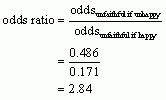
If a woman reported being unhappy in her relationship, the odds of her being unfaithful were 2.84 times higher than if she reported happiness.
For puzzle 2:
The values that we need to answer this puzzle can be found in Table 13.8. We want to know how much more likely a woman is to be unfaithful if she incompatible rather than compatible in her relationship (or vice versa). To begin with, we want to know the odds of a woman being unfaithful given she feels incompatible, which will be the probability of a woman who feels incompatible being unfaithful divided by the probability of a woman who feels incompatible being faithful:

Next, we calculate the odds that a woman was unfaithful given she felt compatible:

We can then calculate the odds ratio as the odds of being unfaithful if a woman reported feeling incompatible divided by the odds of a woman being unfaithful but reporting feeling compatible:
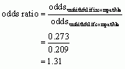
If a woman reported feeling incompatible in her relationship, the odds of her being unfaithful were only 1.31 times higher than if she reported feeling compatible.
For puzzle 3:
The values that we need to answer this puzzle can be found in Table 13.9. This time let’s calculate how much more likely a man is to be faithful if he feels compatible rather than incompatible with his partner (or vice versa). To begin with, we want to know the odds of a man being faithful given he feels compatible with his partner, which will be the probability of a man feeling compatible and being faithful divided by the probability of a man feeling compatible and being unfaithful:

Next, we calculate the odds that a man was faithful given he felt incompatible with his partner:

The odds ratio is the odds of a man who feels compatible with his partner being faithful divided by the odds of a man who feels incompatible with his partner being faithful.
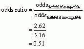
This ratio tells us that a man who felt compatible with his partner was about half as likely (0.51) to be faithful (than unfaithful) than a man who felt incompatible with his partner.
Puzzle 7
Using the data in Table 13.4 (in the book chapter and reproduced below), compute the Pearson correlation, confidence interval, and t-statistic for the relationship between Neuroticism and each of Rewards, Costs, Ideal and Alternatives.
Table 13.4 (reproduced): Data on neuroticism and relationship commitment based on Kurdek (1997)

Neuroticism and Rewards
Let’s start with the Pearson correlation between Neuroticism and Rewards. First we need to calculate the cross-product deviations so that we can calculate the covariance (Table 7).
Table 7: Calculating cross-product deviations between Neuroticism and Rewards

We calculate the covariance using the equation:

Now we can calculate the Pearson correlation coefficient using the equation:
![]()
Therefore, the Pearson correlation coefficient between Neuroticism and Rewards was -0.73. This is quite a large negative effect and means that the more neurotic the person, the less rewards they felt they received from their relationship.
Next let’s calculate the t-statistic:
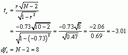
Now we have to look up the critical value for a t-distribution (Section A.2 in the book) with 8 degrees of freedom. Reading across the row for 8 degrees of freedom in the t-distribution table, we can see that the critical value for a two-tailed test with a p equal to 0.05 is 2.306. The value of t that we observed was -3.01, and we can ignore the minus sign because that just tells us the direction of the effect. The question is whether our observed value of -3.01 is bigger than the critical value of 2.306, which it is, suggesting that there is a significant negative relationship between neuroticism and how rewarding you perceive your relationship to be; i.e., the more neurotic you are, the less rewarding you perceive your relationship to be.
Finally, the puzzle asks us to calculate the confidence interval for r. To do this we need to convert r to a z-score using the following equation:
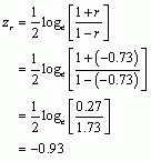
We also need to calculate ![]() using the following equation:
using the following equation:
![]()
We can now calculate the confidence interval using the equation:

![]()
We can now convert the values from z back to r using this equation:
![]()

The confidence interval is -0.93 to -0.18, which does not contain zero. This suggests that there is a significant negative relationship between neuroticism and rewards, i.e., the more neurotic you are the less likely you are to perceive your relationship as rewarding.
Neuroticism and Costs
To calculate the Pearson correlation between Neuroticism and Costs, first we need to calculate the cross-product deviations so that we can calculate the covariance (Table 8).
Table 8: Calculating cross-product deviations between Neuroticism and Costs

We calculate the covariance using the equation:
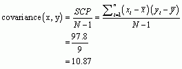
Now we can calculate the Pearson correlation coefficient using the equation:
![]()
Therefore, the Pearson correlation coefficient between Neuroticism and Costs was 0.68. This is quite a large positive effect and means that the more neurotic the person, the more costs they felt were associated with their relationship.
Next let’s calculate the t-statistic:

Now we have to look up the critical value for a t-distribution with 8 degrees of freedom (Section A.2 in the book). Reading across the row for 8 degrees of freedom in the t-distribution table, we can see that the critical value for a two-tailed test with a p equal to 0.05 is 2.306. The value of t that we observed was 2.60, which is slightly bigger than the critical value of 2.306, suggesting that there is a significant positive relationship between neuroticism and the costs you perceive your relationship to have, i.e., the more neurotic you are, the more costs you perceive your relationship to have.
Finally, the puzzle asks us to calculate the confidence interval for r. To do this we need to convert r to a z-score using the following equation:
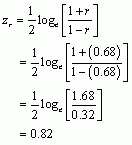
We also need to calculate ![]() using the following equation:
using the following equation:
![]()
We can calculate the confidence interval using the equation:

![]()
We can convert the values from z back to r using this equation:
![]()

The confidence interval is 0.08 to 0.92, which does not contain zero. This suggests that there is a significant positive relationship between neuroticism and costs, i.e., the more neurotic you are the more likely you are to perceive your relationship as having more costs.
Neuroticism and Ideal
To calculate the Pearson correlation between Neuroticism and Ideal, first we need to calculate the cross-product deviations so that we can calculate the covariance (Table 9).
Table 9: Calculating cross-product deviations between Neuroticism and Ideal

We calculate the covariance using the equation:
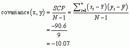
Now we can calculate the Pearson correlation coefficient using the equation:
![]()
Therefore, the Pearson correlation coefficient between Neuroticism and Ideal was -0.62![]() This is a medium negative effect and means that the more neurotic the person, the less ideal they felt their relationship was.
This is a medium negative effect and means that the more neurotic the person, the less ideal they felt their relationship was.
Next let’s calculate the t-statistic:
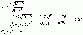
Now we have to look up the critical value for a t-distribution with 8 degrees of freedom. Reading across the row for 8 degrees of freedom in the t-distribution table, we can see that the critical value for a two-tailed test with a p equal to 0.05 is 2.306. The value of t that we observed was -2.25, which is slightly less than the critical value of 2.306, suggesting that there is not a significant relationship between neuroticism and how ideal you perceive your relationship to be.
Finally, the puzzle asks us to calculate the confidence interval for r. To do this we need to convert r to a z-score using the following equation:

We also need to calculate ![]() using the following equation:
using the following equation:
![]()
We can calculate the confidence interval using the equation:

![]()
We can convert the values from z back to r using this equation:
![]()

The confidence interval is -0.90 to 0.02, which contains zero, suggesting that there is not likely to be a significant relationship between the variables Neuroticism and Ideal.
Neuroticism and Alternatives
To calculate the Pearson correlation between Neuroticism and Alternatives, first we need to calculate the cross-product deviations so that we can calculate the covariance (Table 10).
Table 10: Calculating cross-product deviations between Neuroticism and Alternatives

We calculate the covariance using the equation:
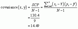
Now calculate the Pearson correlation coefficient using the equation:
![]()
Therefore, the Pearson correlation coefficient between Neuroticism and Alternatives was 0.72. This is a large positive effect, suggesting that the more neurotic the person, the more they searched for alternative partners.
Next let’s calculate the t-statistic:

Now we have to look up the critical value for a t-distribution with 8 degrees of freedom. Reading across the row for 8 degrees of freedom in the t-distribution table, we can see that the critical value for a two-tailed test with a p equal to 0.05 is 2.306. The value of t that we observed was 2.96, which is bigger than the critical value of 2.306, suggesting that there was a significant relationship between neuroticism and alternatives.
Finally, the puzzle asks us to calculate the confidence interval for r. To do this we need to convert r to a z-score using the following equation:
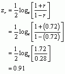
We also need to calculate ![]() using the following equation:
using the following equation:
![]()
We can calculate the confidence interval using the equation:

![]()
We can now convert the values from z back to r using this equation:
![]()

The confidence interval is 0.17 to 0.93, which does not contain zero, suggesting that there is likely to be a significant positive relationship between the variables Neuroticism and Alternatives.
Puzzle 8
Using the data in Table 13.4 (in the book), compute the Pearson correlation, confidence interval, and t-statistic for the relationship between Rewards and each of Costs, Ideal and Alternatives.
Remember that we’re using the data in Table 13.4 (which was reproduced in the answer to puzzle 7).
Rewards and Costs
Let’s start with the Pearson correlation between Rewards and Costs. First we need to calculate the cross-product deviations so that we can calculate the covariance (Table 11).
Table 11: Calculating cross-product deviations between Rewards and Costs

We calculate the covariance using the equation:
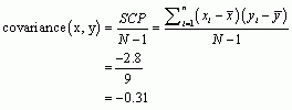
Now we can calculate the Pearson correlation coefficient using the equation:
![]()
Therefore, the Pearson correlation coefficient between Rewards and Costs was ![]() . This is a very small negative effect and means that the more rewards a person felt they received from their relationship, the less costly they felt their relationship was.
. This is a very small negative effect and means that the more rewards a person felt they received from their relationship, the less costly they felt their relationship was.
Next let’s calculate the t-statistic:
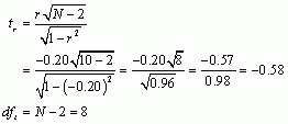
Now we have to look up the critical value for a t-distribution with 8 degrees of freedom. Reading across the row for 8 degrees of freedom in the t-distribution table, we can see that the critical value for a two-tailed test with a p equal to 0.05 is 2.306. The value of t that we observed was -0.58, and we can ignore the minus sign because that just tells us the direction of the effect. The observed value of -0.58 is not bigger than the critical value of 2.306, suggesting that there was not a significant relationship between how many rewards people felt they gained from their relationship and the costs they felt were involved with their relationship.
Finally, the puzzle asks us to calculate the confidence interval for r. To do this we need to convert r to a z-score using the following equation:
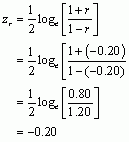
We also need to calculate ![]() using the following equation:
using the following equation:
![]()
We can calculate the confidence interval using the equation:

![]()
We can convert the values from z back to r using this equation:
![]()

The confidence interval is -0.74 to 0.50, which does contain zero. This again suggests that there is not a significant relationship between Rewards and Costs.
Rewards and Ideal
To calculate the Pearson correlation between Rewards and Ideal, first we need to calculate the cross-product deviations so that we can calculate the covariance (Table 12).
Table 12: Calculating cross-product deviations between Rewards and Ideal

We calculate the covariance using the equation:
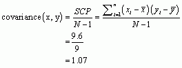
Now we can calculate the Pearson correlation coefficient using the equation:
![]()
Therefore, the Pearson correlation coefficient between Rewards and Ideal was ![]() . This is a medium large effect and means that the more rewards a person felt they received from their relationship, the more ideal they felt their relationship was, which makes sense!
. This is a medium large effect and means that the more rewards a person felt they received from their relationship, the more ideal they felt their relationship was, which makes sense!
Next let’s calculate the t-statistic:

Now we have to look up the critical value for a t-distribution with 8 degrees of freedom. Reading across the row for 8 degrees of freedom in the t-distribution table, we can see that the critical value for a two-tailed test with a p equal to 0.05 is 2.306. The value of t that we observed was 2.59, which is bigger than the critical value of 2.306, suggesting that there was a significant relationship between how many rewards people felt they gained from their relationship and how ideal they felt their relationship was.
Finally, the puzzle asks us to calculate the confidence interval for r. To do this we need to convert r to a z-score using the following equation:
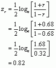
We also need to calculate ![]() using the following equation:
using the following equation:
![]()
We can calculate the confidence interval using the equation:

![]()
We can convert the values from z back to r using this equation:
![]()

The confidence interval is 0.08 to 0.92, which does not cross zero and therefore indicates that there is a significant relationship between Rewards and Ideal.
Rewards and Alternatives
To calculate the Pearson correlation between Rewards and Alternatives, first we need to calculate the cross-product deviations so that we can calculate the covariance (Table 13).
Table 13: Calculating cross-product deviations between Rewards and Alternatives

We calculate the covariance using the equation:
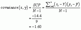
Now we can calculate the Pearson correlation coefficient using the equation:
![]()
Therefore, the Pearson correlation coefficient between Rewards and Alternatives was ![]() . This is a large negative effect and means that the more rewards a person felt they received from their relationship, the less likely they were to look for alternatives.
. This is a large negative effect and means that the more rewards a person felt they received from their relationship, the less likely they were to look for alternatives.
Next, let’s calculate the t-statistic:
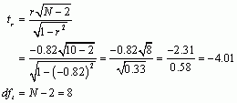
Now we have to look up the critical value for a t-distribution with 8 degrees of freedom. Reading across the row for 8 degrees of freedom in the t-distribution table, we can see that the critical value for a two-tailed test with a p equal to 0.05 is 2.306. The value of t that we observed was -4.01 , and we can ignore the minus sign because that just tells us the direction of the effect. The observed value of -4.01 is bigger than the critical value of 2.306, suggesting that there is a significant relationship between how many rewards people felt they gained from their relationship and how likely they were to search for alternatives; i.e., the more rewards they felt they received from their relationship, the less they were open to alternatives.
Finally, the puzzle asks us to calculate the confidence interval for r. To do this we need to convert r to a z-score using the following equation:
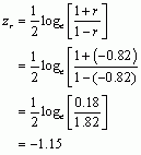
We also need to calculate ![]() using the following equation:
using the following equation:
![]()
We can calculate the confidence interval using the equation:

![]()
We can convert the values from z back to r using this equation:
![]()

The confidence interval is -0.96 to -0.38, which does not contain zero and again suggests that there is a significant relationship between Rewards and Alternatives.
Puzzle 9
Using the data in Table 13.4 (in the book), compute the Pearson correlation, confidence interval, and t-statistic for the relationship between Costs and each of Ideal and Alternatives.
Remember that we’re using the data in Table 13.4 (which was reproduced in the answer to puzzle 7).
Costs and Ideal
To calculate the Pearson correlation between Costs and Ideal, first we need to calculate the cross-product deviations so that we can calculate the covariance (Table 14).
Table 14: Calculating cross-product deviations between Costs and Ideal

We calculate the covariance using the equation:
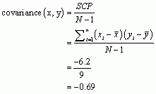
Now we can calculate the Pearson correlation coefficient using the equation:
![]()
Therefore, the Pearson correlation coefficient between Costs and Ideal was ![]() . This is a medium negative effect and means that the more costs a person felt were associated with their relationship, the less ideal they viewed their relationship to be.
. This is a medium negative effect and means that the more costs a person felt were associated with their relationship, the less ideal they viewed their relationship to be.
Next, let’s calculate the t-statistic:
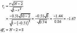
Now we have to look up the critical value for a t-distribution with 8 degrees of freedom. Reading across the row for 8 degrees of freedom in the t-distribution table, we can see that the critical value for a two-tailed test with a p equal to 0.05 is 2.306. The value of t that we observed was ![]() , and we can ignore the minus sign because that just tells us the direction of the effect. The question is whether our observed value of
, and we can ignore the minus sign because that just tells us the direction of the effect. The question is whether our observed value of ![]() is bigger than the critical value of 2.306, which it is not, suggesting that there was not a significant relationship between the costs people felt were associated with their relationship and how ideal they viewed their relationship to be.
is bigger than the critical value of 2.306, which it is not, suggesting that there was not a significant relationship between the costs people felt were associated with their relationship and how ideal they viewed their relationship to be.
Finally, the puzzle asks us to calculate the confidence interval for r. To do this we need to convert r to a z-score using the following equation:
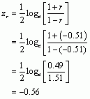
We also need to calculate ![]() using the following equation:
using the following equation:
![]()
We can calculate the confidence interval using the equation:

![]()
We can convert the values from z back to r using this equation:
![]()

The confidence interval is -0.86 to 0.18, which crosses zero and therefore suggests that there is not a significant relationship between Costs and Ideal.
Costs and Alternatives
To calculate the Pearson correlation between Costs and Alternatives, first we need to calculate the cross-product deviations so that we can calculate the covariance (Table 15).
Table 15: Calculating cross-product deviations between Costs and Alternatives

We calculate the covariance using the equation:
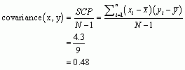
Now we can calculate the Pearson correlation coefficient using the equation:
![]()
Therefore, the Pearson correlation coefficient between Costs and Alternatives was 0.28. This is a very small positive effect and means that the more costs a person felt were associated with their relationship the more open they were to alternatives.
Next let’s calculate the t-statistic:
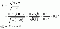
Now we have to look up the critical value for a t-distribution with 8 degrees of freedom. Reading across the row for 8 degrees of freedom in the t-distribution table, we can see that the critical value for a two-tailed test with a p equal to 0.05 is 2.306. The value of t that we observed was 0.84, which is smaller than the critical value of 2.306, suggesting that there was not a significant relationship between the number of costs people felt were associated with their relationship and how open to alternatives they were.
Finally, the puzzle asks us to calculate the confidence interval for r. To do this we need to convert r to a z-score using the following equation:
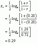
We also need to calculate ![]() using the following equation:
using the following equation:
![]()
We can calculate the confidence interval using the equation:

![]()
We can convert the values from z back to r using this equation:
![]()

The confidence interval is -0.42 to 0.78, which crosses zero and therefore suggests that there is not a significant relationship between Costs and Alternatives.
Puzzle 10
What is the relationship between covariance and the correlation coefficient?
Both covariance and correlation indicate whether variables are positively or negatively related. However, unlike the correlation coefficient, the covariance is not a standardized measure: it depends upon the scales of measurement and as such you cannot interpret covariance in an objective way – you cannot say whether a covariance is particularly large or small relative to another data set unless both data sets were measured in the same units. We can convert the covariance into the correlation coefficient, which is a standardized measure, by dividing it by the two standard deviations for each variable multiplied together:
![]()
