An Adventure in Statistics: The Reality Enigma
Student Resources
Jig:Saw’s puzzle solutions
Puzzle 1
According to Paul Zak, the hormone oxytocin increases trust in humans. You do an experiment in which groups of people are exposed to oxytocin or not while meeting a stranger. They rate how much they trusted the stranger from 0 (no trust) to 10 (complete trust). The oxytocin group had a mean trust of M = 7.45 (SD = 2.67) and the non-exposed group had a mean trust of M = 5.13 (SD = 1.12). What is Cohen’s d for this difference? (Compute it using the pooled variance estimate as well as using the control group variability.)
Cohen’s d using the control group standard deviation is 2.07:
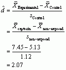
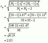
This value means that if a person were exposed to oxytocin their trust rating of a stranger would increase by 2.07 standard deviations, which is a very large effect. If the groups are independent then you can pool the standard deviations. Unfortunately, I’m an idiot and didn’t tell you the group sample sizes, and you need these to put into the equation, so it’s impossible to answer this question given the information provided. However, let’s assume, as in Table 11.3 in the book, that there were 50 people in each group. The pooled standard deviation would be 2.05:
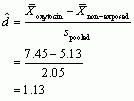
The Cohen’s d using the pooled standard deviation is 1.13:
Puzzle 2
In a different version of the oxytocin study, participants are simply classified according to whether they trusted the stranger or not. The data are in Table 11.3 (in the book and reproduced below). What is the odds ratio for these data?
First, we calculate the odds that a person trusted a stranger after being exposed to oxytocin:

Next, we calculate the odds that a person trusted a stranger when not exposed to oxytocin:

The odds ratio is the odds of trusting a stranger after oxytocin divided by the odds of trusting a stranger after no oxytocin. This ratio tells us that people who were exposed to oxytocin were twice as likely to trust a stranger than people who were not exposed to oxytocin.
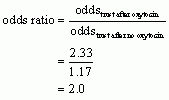
Table 11.3 (reproduced): Number of people who trusted a stranger depending on whether they were exposed to oxytocin or not during the meeting

Puzzle 3
For the data in Table 11.3 (in the book and reproduced above), use Bayes’ theorem to compute the conditional probability of trusting the stranger given you received oxytocin, p(trust|oxytocin). What is the conditional probability of trusting given that you didn’t receive oxytocin, p(trust|no oxytocin)?

Therefore, the conditional probability of trusting a stranger given you received oxytocin is quite high: 0.7, or a 70% chance.

Therefore, the conditional probability of trusting a stranger given you did not receive oxytocin is 0.54, or a 54% chance.
Puzzle 4
For the data in Table 11.3 (in the book and reproduced in puzzle 2), what are the posterior odds of trusting the stranger when given oxytocin than when not?
The posterior odds are the ratio of the posterior probability for one hypothesis to another. In this example it would be the ratio of the probability that a person trusted the stranger given they received oxytocin (which we have already calculated in puzzle 3 to be 0.70) to the probability that they trusted the stranger given they received no oxytocin (which we have already calculated in puzzle 3 to be 0.54). The value turns out to be 1.30, which means that the probability that you were exposed to oxytocin if you trusted the stranger is 1.3 times higher than the probability that you were not exposed to oxytocin if you trusted the stranger.
![]()
Puzzle 5
What does a Bayes factor tell us?
The Bayes factor is the ratio of the probability of the data given the alternative hypothesis to that of the data given the null hypothesis. A Bayes factor less than 1 supports the null hypothesis (it suggests the data are more likely given the null hypothesis than the alternative hypothesis); conversely, a Bayes factor greater than 1 suggests that the observed data are more likely given the alternative hypothesis than the null. Values between 1 and 3 are considered evidence for the alternative hypothesis that is ‘barely worth mentioning’, values between 3 and 10 are considered to indicate evidence for the alternative hypothesis that ‘has substance’, and values greater than 10 are strong evidence for the alternative hypothesis.
Puzzle 6
Describe the differences between NHST and Bayesian hypothesis testing.
- NHST uses two competing hypotheses: one says that an effect exists (the alternative hypothesis) and the other says that an effect doesn’t exist (the null hypothesis). You compute a test statistic that represents the alternative hypothesis and calculate the probability that you would get a value at least as big as the one you have if the null hypothesis were true. If this probability is less than 0.05 scientists reject the idea that there is no effect and conclude that they have a statistically significant finding. If the probability is greater than 0.05 they do not reject the idea that there is no effect, and conclude that they have a non-significant finding. Bayesian hypothesis testing, on the other hand, is based on looking at the probability of the alternative hypothesis given the data and comparing this to the probability of the null hypothesis given the data. Alternatively, Bayes factors can be used to compare the probability of the observed data given the alternative hypothesis to the probability of the observed data given the null hypothesis. As such, Bayesian hypothesis testing does not rely on arbitrary criteria for ‘significance’; instead, you interpret the weight of evidence for one hypothesis over another.
- Bayesian approaches aim to evaluate the evidence for the null hypothesis, so, unlike NHST, they allow you to draw conclusions about the likelihood that the null hypothesis is true.
- In NHST, the significance of a test statistic is directly linked to the sample size. The same effect will have different p-values in different-sized samples: small differences can be deemed ‘significant’ in large samples, and large effects might be deemed ‘non-significant’ in small samples. In Bayesian analysis, sample size is not an issue, except that the more data you collect, the more evidence you use to update your beliefs about the alternative and null hypothesis.
- When conducting NHST you need to determine how much data to collect before performing your analysis; however, you do not need to do this before performing Bayesian analysis. This is because Bayesian analysis is not based on long-run probabilities, so it does not matter when you stop collecting data or what your rule for collecting data is, because any new data relevant to your hypothesis can be used to update your prior beliefs in the null and alternative hypotheses.
Puzzle 7
What is the difference between a confidence interval and a credible interval?
A 95% confidence interval is set so that before the data are collected there is a long-run probability of 0.95 (or 95%) that the interval will contain the true value of the parameter. This means that in 100 random samples, the intervals will contain the true value in 95 of them but won’t in 5. Once the data are collected, your sample is either one of the 95% that produces an interval containing the true value, or one of the 5% that does not. In other words, having collected the data, the probability of the interval containing the true value of the parameter is either 0 (it does not contain it) or 1 (it does contain it), but you do not know which. A credible interval is different in that it reflects the plausible probability that the interval contains the true value. For example, a 95% credible interval has a plausible 0.95 probability of containing the true value.
Puzzle 8
What is a meta-analysis?
Meta-analysis is where effect sizes from different studies testing the same hypothesis are combined to get a better estimate of the size of the effect in the population.
Puzzle 9
Zach stole some glasses to help with emotion detection. These were tested on 252 people. Some wore the glasses, some didn’t, and they had to identify a stranger’s emotion from their facial expression. The numbers correct and incorrect in each group are in Table 11.4 (in the book and reproduced below) What is the odds ratio for these data?
First, we calculate the odds that a person correctly identified emotion and wore the glasses:

Next, we calculate the odds that a person correctly identified emotion and didn’t wear the glasses:

The odds ratio is the odds of correctly identifying emotion while wearing the glasses divided by the odds of correctly identifying emotion while not wearing the glasses. This ratio tells us that people who wore the glasses were 0.63 times as likely to identify emotion correctly than people who did not wear the glasses.
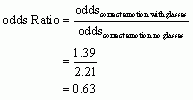
Table 11.4 (reproduced): Number of people who correctly identified a stranger’s emotion depending on whether they were wearing emotion detection glasses or not

Puzzle 10
For the data in Table 11.4 (in the book and reproduced above) use Bayes’ theorem to compute the conditional probability of correctly identifying an emotion given you wore the glasses, p(correct|glasses). What is the conditional probability of being correct given that you didn’t wear the glasses, p(correct|no glasses)?
The conditional probability of correctly identifying emotion given you wore the glasses is 0.58, or a 58% chance:

The conditional probability of correctly identifying emotion given you did not wear the glasses is 0.69, or a 69% chance.

Puzzle 11
For the data in Table 11.4 (in the book and reproduced in puzzle 9), what are the posterior odds of correctly identifying emotion in the stranger when wearing the glasses than when not?
The posterior odds are the ratio of the posterior probability for one hypothesis to another. In this example it would be the ratio of the probability that a person correctly identified emotion given they wore the glasses (which we have already calculated in puzzle 10 to be 0.58) to the probability that they correctly identified emotion given that they did not wear the glasses (which we have already calculated in question 10 to be 0.69). The value turns out to be 0.84 which means that the probability that you wore glasses if you correctly identified the emotion is 0.84times the probability that you didn’t wear glasses if you correctly identified the emotion. In other words, the glasses didn’t help to identify emotions!
![]()
