Part 1: Cross-Tabulations

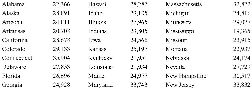
The American Community Survey provides information on, among other topics, 2007 per capita income¹. These data are provided below for 30 U.S. states.

1. In order to construct a bivariate table, we need to reclassify these data into more broadly defined categories. Develop a coding scheme which permits you to classify each of the above states into one of four categories: West, Midwest, Northeast, and South. How many states fall into each of these categories?
2. Now that you have grouped states by their geographic location, do the same for per capita income. Within each of the four geographic clusters, assign each state into one of two categories based on the level of per capita income: below $25,000 or above $25,000. The end result should be a bivariate table with 4 columns and 2 rows (assuming that per capita income is the row variable). Display this table.
3. Next, we need to percentage the table presented in Question #2. Following the conventions established in Chapter 10, percentage the table within each column.
4. Considering your answer to Question #3, make the appropriate comparisons of the percentages to determine if there appears to be a weak, moderate, or strong relationship between geographic location and per capita income.
5. Is it possible to determine the direction of the relationship between geographic location and per capita income? Why or why not?
6. Could the relationship between geographic location and per capita income be spurious? Why or why not?
7. Is it possible that one or more intervening variables could affect your conclusion from Question #4? Why or why not?
8. Upon reexamining your results, you decide to further collapse some of the geographic categories you developed earlier. Collapse West and Midwest into one category and Northeast and South in a second category. Display the bivariate table for these data.
9. Next, we need to percentage the table presented in Question #2. Following the conventions established in Chapter 10, percentage the table within each column.
10. Discuss your results from Question #9. Why did these differ so drastically from those in Question #3?
11. In general, do the conclusions that we are able to draw from bivariate tables depend in part on the specification of the categories for each of the variables? Why or why not?
12. Assume that a person’s income is directly dependent on the state they live in. What is the independent variable in this relationship?
13. Define: Cross-tabulation.

¹http://factfinder.census.gov/jsp/saff/SAFFInfo.jsp?_pageId=sp1_acs&_submenuId=

Part 2: Chi-Square and Measures of Association

In the late summer of 2008, a brief war broke out between the two countries of Russia and Georgia. Suppose you are a researcher interested in nationalistic attitudes in these two countries. You decided to use data from the World Values Survey, which is available at the following URL: http://www.worldvaluessurvey.org/. The data of interest are presented below on Russian respondents.

1. Identify the dependent variable.
2. What is the total sample size?
3. Calculate the values of the row and column marginals.
4. Calculate the expected frequencies for each cell.
5. Provide an interpretation of the expected cell frequencies. What do these quantities represent?
6. Following the example in Chapter 11, calculate the chi-square statistic.
7. Calculate the number of degrees of freedom for this particular example.
8. Using the table in the back of your textbook, what is the critical value for this chi-square test? (Note: use the .05 column)
9. On the basis of your work in Questions #6-8, conclude whether your results are statistically significant. Provide evidence for your conclusion.
10. Return to the original data. Exactly 940 persons between the ages of 15 and 29 indicated that they were "quite proud of their nationality. Suppose for the moment that only 840 persons between the ages of 15 and 29 were "quite proud" of their nationality. Keeping the other cells as they were originally, recalculate the value of the chi-square statistic and determine whether it is statistically significant.
11. Explain why adjusting only one cell in Question #10 resulted in a different conclusion.
12. As the number of degrees of freedom increases, how does this change the Chi-square distribution?
13. When two variables are not associated what can we say about their relationship?
14. Identify the independent variable.
15. What is the total sample size?
16. Calculate the values of the row and column marginals.
17. Assume for the moment that both variables - age and national pride - are nominal level variables. If both were nominal level variables, which measure of association would be appropriate for these data?
18. Calculate the measure of association you identified in Question #18.
19. Explain why, in terms of calculating the values of E1 and E2, you arrived at the answer that you did in Question #19.
20. Of course, if we were to assume that age and national pride were nominal level variables, we would be mistaken. Identify the level of measurement for these two variables and suggest an appropriate measure of association to gauge the relationship between these two variables.
21. One measure of association that we might employ to assess the relationship between age and national pride is that of gamma, as it was introduced in Chapter 11. Begin by calculating the number of same ordered pairs.
22. Next, calculate the number of inverse order pairs.
23. Finally, calculate the value gamma. Interpret this quantity.
24. According to the material presented in Chapter 11, what are the lowest and highest possible values for gamma?
25. In light of the results thus far, what would happen if out of curiosity we used national pride as our independent variable. Would this affect the calculation of gamma? Why or why not?